Chapter 6: Investment appraisal under uncertainty
Chapter learning objectives
Upon completion of this chapter you will be able to:
- distinguish between risk and uncertainty in investment appraisal
- define sensitivity analysis and discuss its usefulness in assisting investment decisions
- apply sensitivity analysis to investment projects and explain the meaning of the findings
- define an expected value (EV) and discuss the usefulness of probability analysis in assisting investment decisions
- apply probability analysis to investment projects and explain the meaning of the findings
- discuss the use of simulation to take account of risk and uncertainty in investment appraisal
- discuss the use of adjusted payback in investment appraisal
- calculate the discounted payback and discuss its usefulness as an investment appraisal method
- explain the principle of adjusting discount rates to take account of risk.
1 Risk and uncertainty
The difference between risk and uncertainty
Investment appraisal faces the following problems:
- all decisions are based on forecasts
- all forecasts are subject to uncertainty
- this uncertainty needs to be reflected in the financial evaluation.
 The decision maker must distinguish between:
- risk – quantifiable – possible outcomes have associated probabilities, thus allowing the use of mathematical techniques
- uncertainty – unquantifiable – outcomes cannot be mathematically modelled.
In investment appraisal the areas of concern are therefore the accuracy of the estimates concerning:
- project life
- predicted cash flows and associated probabilities
- discount rate used.
Incorporating risk and uncertainty
2 Sensitivity analysis
- Sensitivity analysis typically involves posing 'what if?' questions.
- For example, what if demand fell by 10% compared to our original forecasts? Would the project still be viable?
- Ideally we want to know how much demand could fall before the project should be rejected or, equivalently, the breakeven demand that gives an NPV of zero. We could then assess the likelihood of forecast demand being that low.
Calculating sensitivity
This maximum possible change is often expressed as a percentage:

This would be calculated for each input individually.
 The lower the sensitivity margin, the more sensitive the decision tothe particular parameter being considered, i.e. small changes in theestimate could change the project decision from accept to reject.
NB Because we will need the PV of each cash flow separately,the following tabular approach is the preferred layout for the NPVcalculation:


 Test your understanding 1 – Sensitivity analysis
An investment of $40,000 today is expected to give rise to annualcontribution of $25,000. This is based on selling one product, with asales volume of 10,000 units, selling price of $12.50 and variable costsper unit of $10. Annual fixed cost of $10,000 will be incurred for thenext four years; the discount rate is 10%.
Required:
(a)Calculate the NPV of this investment.
(b)Calculate the sensitivity of your calculation to the following:
(i)initial investment
(ii) selling price per unit
(iii)sales volume
(iv)fixed costs
(v) discount rate


 Test your understanding 2 – Sensitivity analysis
Bacher Co is considering investing $500,000 in equipment to producea new type of ball. Sales of the product are expected to continue forthree years, at the end of which the equipment will have a scrap valueof $80,000. Sales revenue of $600,000 pa will be generated at a variablecost of $350,000. Annual fixed costs will increase by $40,000.
(a)Determine whether, on the basisof the estimates given, the project should be undertaken, assuming thatall cash flows occur at annual intervals and that Bacher Co has a costof capital of 15%.
(b)Find the percentage changes required in the following estimates for the investment decision to change:
(i)initial investment
(ii) scrap value
(iii)selling price
(iv)unit variable cost
(v) annual fixed cost
(vi)sales volume
(vii) cost of capital.

Advantages and disadvantages of sensitivity analysis
Advantages
- simple
- provides more information to allow management to make subjective judgements
- identifies critical estimates.
Disadvantages:
- assumes variables change independently of each other
- does not assess the likelihood of a variable changing
- does not directly identify a correct decision.

 Advantages and disadvantages of sensitivity analysis
Strengths of sensitivity analysis
- No complicated theory to understand.
- Information will be presented to management in a form which facilitates subjective judgement to decide the likelihood of the various possible outcomes considered.
- Identifies areas which are crucial to the success of the project. If the project is chosen, those areas can be carefully monitored.
- Indicates just how critical are some of the forecasts which are considered to be uncertain.
Weaknesses of sensitivity analysis
- It assumes that changes to variables can be made independently, e.g. material prices will change independently of other variables. This is unlikely. If material prices went up the firm would probably increase selling price at the same time and there would be little effect on NPV. A technique called simulation (see later) allows us to change more than one variable at a time.
- It only identifies how far a variable needs to change. It does not look at the probability of such a change. In the above analysis, sales volume appears to be the most crucial variable, but if the firm were facing volatile raw material markets a 65% change in raw material prices would be far more likely than a 29% change in sales volume.
- It is not an optimising technique. It provides information on the basis of which decisions can be made. It does not point directly to the correct decision.


 Sensitivity analysis - the certainty equivalent approach
An alternative method of performing sensitivity analysis is the certainty equivalent approach.
With this approach the cash flows of the project are calculated asper normal but then adjusted downwards by a certain equivalent factor.This in effect decreases the cash flow. The cash flows are thendiscounted at the risk-free rate.
Illustration
Total NPV = $407,000
In practice the major problem is that the use of certainty equivalents is subjective.

3 Probability analysis
When there are several possible outcomes for a decision andprobabilities can be assigned to each, a probability distribution ofexpected cash flows can often be estimated, recognising there areseveral possible outcomes, not just one. This could then be used to:
(1)Calculate an expected value (EV);
(2)Measure risk by:
(a)calculating the worst possible outcome and its probability;
(b)calculating the probability that the project will fail (for example, that a negative NPV will result);
(c)assessing the standard deviation of the outcomes.
 The EV is the weighted average of all the possible outcomes, with the weightings based on the probability estimates.
 The standard deviation is a statistical measure of the variability of adistribution around its mean (i.e. it measures the dispersion ofpossible outcomes about the EV). The tighter the distribution, the lowerthis measure will be. It is a measure of risk – the wider thedispersion the riskier the situation.
Calculating an EV
The formula for calculating an EV is:
EV =∑px
where
p = the probability of an outcome
x = the value of an outcome.
The EV is not the most likely result. It may not even be a possible result, but instead it finds the long-run average outcome.

 Expected values
The EV is the weighted average of the outcomes, with the weightings based on the probability estimates.
The EV does not necessarily represent what the outcome will be, nordoes it represent the most likely result. What it really represents isthe average pay-off per occasion if the project were repeated many times(i.e. a 'long-run' average).
There are two main problems with using EV to make decisions in this way:
- The project will only be carried out once. It could result in a sizeable loss and there may be no second chance to win our money back.
- The probabilities used are simply subjective estimates of our belief, on a scale from 0 to 1. There is probably little data on which to base these estimates.


 Test your understanding 3 – Expected values
A firm has to choose between three mutually exclusive projects, theoutcomes of which depend on the state of the economy. The followingestimates have been made:

Determine which project should be selected on the basis of expected market values.

Using EVs in larger NPV calculations
The EV technique can be used to simplify the available data in a larger investment appraisal question.

 Test your understanding 4 – Expected values in larger NPV
Dralin Co is considering an investment of $460,000 in a non-currentasset expected to generate substantial cash inflows over the next fiveyears. Unfortunately the annual cash flows from this investment areuncertain, but the following probability distribution has beenestablished:
At the end of its five-year life, the asset is expected to sell for $40,000. The cost of capital is 5%.
Should the investment be undertaken?

Using EVs with decision matrices
EVs are also used to deal with situations where the same conditionsare faced many times. The problems involve construction of a 'decisionmatrix'.

 Using EVs with decision matrices
Illustration – Using expected values with decision matrices
A newsagent sells a weekly magazine which advertises localsecond-hand goods. The owner can buy the magazines for 15c each and sellthem at the retail price of 25c. At the end of each week unsoldmagazines are obsolete and have no value.
The owner estimates a probability distribution for weekly demand which looks like this:
(a)What is the EV of demand?
(b)If the owner is to order a fixedquantity of magazines per week how many should that be? Assume noseasonal variations in demand.
Solution
(a)EV of demand = (10 × 0.20) + (15 × 0.55) + (20 × 0.25) = 15.25 units per week.
(b)Step 1: Set up a decision matrix of possible strategies (numbers bought) and possible demand, as follows:
Step 2: The 'payoff' from each combination of action and outcome is then computed:
No sale → loss of 15c per magazine.
Sale → profit of 25c − 15c = 10c per magazine.
- Payoffs are shown for each combination of strategy and outcome:
Workings
(i)If 10 magazines are bought, then 10 are sold no matter how many are demanded and the payoff is always 10 × 10c = 100c.
(ii) If 15 magazines are boughtand 10 are demanded, then 10 are sold at a profit of 10 × 10c = 100c,and 5 are scrapped at a loss of 5 × 15c = 75c, making a net profit of25c.
(iii)The other contributions are similarly calculated.
Step 3: Probabilities are then applied to compute the expected value resulting from each possible course of action.
Alternatively, in the same matrix, probability × payoff can be inserted in each cell and totalled to give the expected payoff.

From this matrix we can see that the best alternative is to buy 15 magazines each week.
What does this EV mean?
It means that if the strategy is followed for many weeks, then on average the profit will be 125c per week.
What actually happens is that eight weeks out of ten the payoff is likely to be 150c and two weeks out of ten it drops to 25c.
This strategy produces the highest long-run profit for the firm.

Strengths and weaknesses of EVs
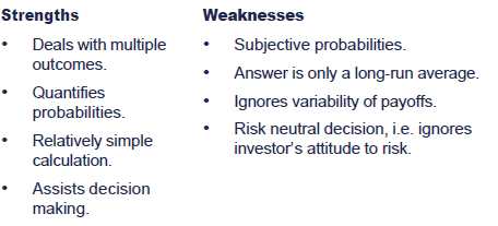
Using EVs as a basis for decision making is appropriate if three conditions are met or nearly met:
- there is a reasonable basis for making the forecasts and estimating the probability of different outcomes
- the decision is relatively small in relation to the business, so risk is small in magnitude
- the decision is for a category of decisions that are often made.
 The EV technique is best suited to a problem which is repetitive and involves relatively small investments.

 Advantages and limitations of EVs
Advantages of EVs
- The technique recognises that there are several possible outcomes and is, therefore, more sophisticated than single value forecasts.
- Enables the probability of the different outcomes to be quantified.
- Leads directly to a simple optimising decision rule by reducing a range of possible outcomes into one number. However, care should be taken (see below)
- Calculations are relatively simple.
Limitations of EVs
- By asking for a series of forecasts the whole forecasting procedure is complicated. Inaccurate forecasting is already a major weakness in project evaluation. The probabilities used are also usually very subjective.
- The EV is merely a weighted average of the probability distribution, indicating the average payoff if the project is repeated many times.
- The EV gives no indication of the dispersion of possible outcomes about the EV. The more widely spread out the possible results are, the more risky the investment is usually seen to be. The EV ignores this aspect of the probability distribution.
- In ignoring risk, the EV technique also ignores the investor's attitude to risk. Some investors are more likely to take risks than others.
Conclusions on EVs
The simple EV decision rule is appropriate if three conditions are met or nearly met:
- there is a reasonable basis for making the forecasts and estimating the probability of different outcomes
- the decision is relatively small in relation to the business. Risk is then small in magnitude
- the decision is for a category of decisions that are often made.
A technique which maximises average payoff is then valid.

4 Further techniques for adjusting for risk and uncertainty
Simulation
Sensitivity analysis considers the effect of changing one variableat a time. Simulation improves on this by looking at the impact of manyvariables changing at the same time.
Using mathematical models, it produces a distribution of thepossible outcomes from the project. The probability of differentoutcomes can then be calculated.
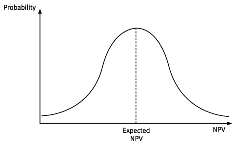
You will never be expected to carry out a simulation exercise in the exam although you may be asked to interpret the output.

 Simulation
The four stages of a simulation exercise
There are four stages involved in carrying out a simulation exercise:
(1)Specify major variables, e.g.:
- Market details
- Investment costs
- Operating costs
(2)Specify the relationships between variables to calculate an NPV, e.g.:
Sales revenue = market size × market share × selling price.
Net cash flow = sales revenue − (variable costs + fixed costs + taxation), etc.
(3)Simulate the environment:
- select different values of each variable within the parameters set and compute an NPV
- repeat the process many times to create a probability distribution of returns.
(4)The results of a simulation exercise will be a probability distribution of NPVs.
- Instead of choosing between expected values, decision makers can now take the dispersion of outcomes and the expected return into account.
Advantages of simulation
The major advantages of simulation are as follows:
- it includes all possible outcomes in the decision-making process
- it is a relatively easily understood technique
- it has a wide variety of applications (inventory control, component replacement, corporate models, etc.).
Drawbacks of simulation
However, it does have some significant drawbacks:
- models can become extremely complex and the time and costs involved in their construction can be more than is gained from the improved decisions
- probability distributions may be difficult to formulate.

Adjusted payback
We looked at the payback form of investment appraisal in the chapter on basic investment appraisal.
One way of dealing with risk is to shorten the payback periodrequired. This places more emphasis on the earlier cash flows, which areconsidered to be less risky.
However, given the disadvantages of payback as a method ofinvestment appraisal, adjusted payback is rarely recommended as a methodof adjusting for risk.
Discounted payback
It is also possible to reflect risk by using discounted cash flowsin the calculation of a discounted payback period. The cash flows arefirst discounted using an appropriate discount rate that reflects therisk profile of the project. The cumulative discounted cash flow canthen be calculated in the same manner as the cumulative cash flow is forthe standard payback calculation.
The discounted payback method has the same advantages anddisadvantages as for the traditional payback method except that theshortcoming of failing to account for the time value of money has beenovercome.

 Illustration 1 Discounted Payback Period
A project with the following cash flows is under consideration:

Cost of capital 8%
Required:
Calculate the Discounted Payback Period.
Solution


Risk-adjusted discount rates
The discount rate we have assumed so far is the rate that reflects either:
- the cost of borrowing funds in the form of a loan rate or
- the underlying required return of the business (i.e. the return required by the shareholder),
- or a mix of both.
If an individual investment or project is perceived to be morerisky than existing investments, the increased risk could be used as areason to adjust the discount rate.
 This is a key concept in investment appraisal. Applying the existingdiscount rate or cost of capital to an investment assumes that theexisting business and gearing risk of the company will remain unchanged.If the project is significant in size and likely to result inadditional risks then a project specific or risk-adjusted discount rateshould be used.
The application of an increased discount rate is often successfulin eliminating marginal projects. The addition to the usual discountrate is called the risk premium. The method used is examined further inthe cost of capital chapter.
Chapter summary
Test your understanding answers

 Test your understanding 1 – Sensitivity analysis
Solution
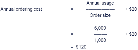
Therefore the decision should be to accept the investment.

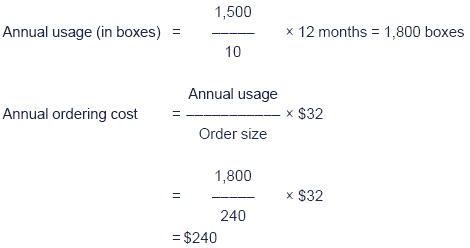
(W1)
If the project NPV is set to zero, the PV of the net cash inflowswould need to be $40,000. Hence the discount factor needed to make theNPV go down to 0 is 40,000÷15,000 = 2.667.
From tables, at four years, the closest annuity rate to 2.667occurs at approximately 18%. This is therefore the breakeven discountrate, i.e. the IRR.
This quick method of finding the IRR will only work if all theinflows are in the form of annuities. Otherwise the usual linearinterpolation route must be followed.


 Test your understanding 2 – Sensitivity analysis
Although part (a) could be completed most efficiently by findingthe PV of net annual inflows ($600,000 − $350,000 − $40,000), i.e. of$210,000, part (b) would be most effectively negotiated if the separatePVs were found.
NPV calculation

The project should, on the basis of these estimates, be accepted.
(a)Sensitivity analysis
(i)Initial investment
For the decision to change, the NPV must fall by $33,000. For this to occur, the cost of the equipment must rise by $33,000.

(ii) Scrap value
If the NPV is to fall by $33,000, the PV of scrap proceeds mustfall by $33,000. The PV of scrap proceeds is currently $53,000. It mustfall by: 33÷53 × 100 = 62.26%, say 62
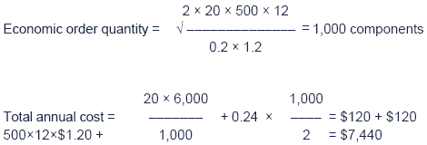
(iii)Selling price
If sales price varies, sales revenue will vary (assuming no effecton demand). If the NPV of the project is to fall by $33,000, theselling price must fall by:
(iv)Unit variable cost
The project's NPV must fall by $33,000 therefore the PV of thevariable costs must rise by $33,000. Since the PV of variable costs is$799,000, a rise of $33,000 is an increase of:

(v) Annual fixed costs
Since the PV of fixed costs is $91,000, a rise of $33,000 is an increase of:

(vi)Sales volume
If sales volume falls, revenue and variable costs fall(contribution falls). If the NPV is to fall by $33,000, volume must fallby:

(vii)Cost of capital
If NPV is to fall, cost of capital must rise. The figure which thecost of capital must rise to, that gives an NPV of zero, is theproject's IRR.
NPV ($000) = − 500 + [210 × 2.210] + [80 × 0.624] = 14 The IRR is alittle more than 17%, possibly 18%, but the formula can be used.
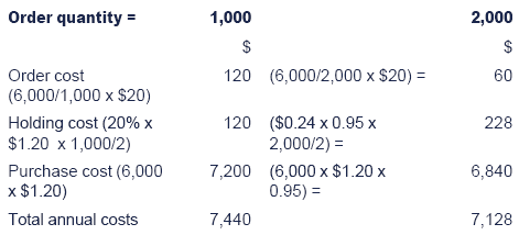
≈ 18.47%, say 18.50%
To find the IRR, which is probably not much above 15%, the NPV at 17% can be found using the summarised cash flows.
The cost of capital would have to increase from 15% to 18½% before the investment decision changes


 Test your understanding 3 – Expected values
Project A

Project B

Project C
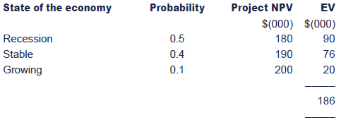
On the basis of expected values Project A should be selected.
However it should be noted that Project A is also the most risky option as it has the widest range of potential outcomes.


 Test your understanding 4 – Expected values in larger NPV
Expected annual cash flows are:

NPV calculation:
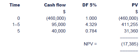
As the ENPV is negative, the project should not be undertaken.
An alternative approach would be to calculate three separate NPVs and then combine them, giving the following figures:
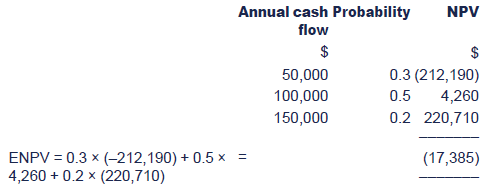
Even though the ENPV is negative these figures show that there is a70% chance of the project giving a positive NPV. Some investors mayconsider the project acceptable on this basis.

|
Created at 5/24/2012 4:12 PM by System Account
(GMT) Greenwich Mean Time : Dublin, Edinburgh, Lisbon, London
|
Last modified at 5/25/2012 12:54 PM by System Account
(GMT) Greenwich Mean Time : Dublin, Edinburgh, Lisbon, London
|
|
|
|
 |
Rating
:
|
 Ratings & Comments
(Click the stars to rate the page) Ratings & Comments
(Click the stars to rate the page)
|
 |
Tags:
|
|
|
|
|