Chapter 8: Working capital management – inventory control

Chapter learning objectives

Upon completion of this chapter you will be able to:

• explain the objective of inventory management
• define and explain lead time and buffer inventory
• explain and apply the basic economic order quantity (EOQ) formula to data provided
• calculate the EOQ taking account of quantity discounts and calculate the financial implications of discounts for bulk purchases
• define and calculate the re-order level where demand and lead time are known
• describe and evaluate the main inventory management systems including Just-In-Time (JIT) techniques
• suggest appropriate inventory management techniques for use in a scenario.

1 The objectives of inventory management

Inventory is a major investment for many companies. Manufacturingcompanies can easily be carrying inventory equivalent to between 50% and100% of the revenue of the business. It is therefore essential toreduce the levels of inventory held to the necessary minimum.

The balancing act

Costs of high inventory levels

Keeping inventory levels high is expensive owing to:

• purchase costs
• holding costs:
  • storage
  • stores administration
  • risk of theft/damage/obsolescence.

Costs of high inventory levels

Carrying inventory involves a major working capital investment andtherefore levels need to be very tightly controlled. The cost is notjust that of purchasing the goods, but also storing, insuring, andmanaging them once they are in inventory.

Purchase costs: once goods are purchased, capital is tied upin them and until sold on (in their current state or converted into afinished product), the capital earns no return. This lost return is anopportunity cost of holding the inventory.

Storage and stores administration: in addition, the goods mustbe stored. The company must incur the expense of renting out warehousespace, or if using space they own, there is an opportunity costassociated with the alternative uses the space could be put to. Theremay also be additional requirements such as controlled temperature orlight which require extra funds.

Other risks: once stored, the goods will need to be insured.Specialist equipment may be needed to transport the inventory to whereit is to be used. Staff will be required to manage the warehouse andprotect against theft and if inventory levels are high, significantinvestment may be required in sophisticated inventory control systems.

The longer inventory is held, the greater the risk that it willdeteriorate or become out of date. This is true of perishable goods,fashion items and high-technology products, for example.

Costs of low inventory levels

If inventory levels are kept too low, the business faces alternative problems:

• stockouts:
  • lost contribution
  • production stoppages
  • emergency orders
• high re-order/setup costs
• lost quantity discounts.

Costs of low inventory levels

Stockout: if a business runs out of a particular product usedin manufacturing it may cause interruptions to the production process– causing idle time, stockpiling of work-in-progress (WIP) or possiblymissed orders. Alternatively, running out of goods held for onward salecan result in dissatisfied customers and perhaps future lost orders ifcustom is switched to alternative suppliers. If a stockout looms, thebusiness may attempt to avoid it by acquiring the goods needed at shortnotice. This may involve using a more expensive or poorer qualitysupplier.

Re-order/setup costs: each time inventory runs out, newsupplies must be acquired. If the goods are bought in, the costs thatarise are associated with administration – completion of a purchaserequisition, authorisation of the order, placing the order with thesupplier, taking and checking the delivery and final settlement of theinvoice. If the goods are to be manufactured, the costs of setting upthe machinery will be incurred each time a new batch is produced.

Lost quantity discounts: purchasing items in bulk will oftenattract a discount from the supplier. If only small amounts are boughtat one time in order to keep inventory levels low, the quantitydiscounts will not be available.

The challenge

The objective of good inventory management is therefore to determine:

• the optimum re-order level – how many items are left in inventory when the next order is placed, and
• the optimum re-order quantity – how many items should be ordered when the order is placed

for all material inventory items.

In practice, this means striking a balance between holding costs on the one hand and stockout and re-order costs on the other.

The balancing act between liquidity and profitability, which might alsobe considered to be a trade-off between holding costs andstockout/re-order costs, is key to any discussion on inventorymanagement.

Terminology

Other key terms associated with inventory management include:

• lead time – the lag between when an order is placed and the item is delivered
• buffer inventory – the basic level of inventory kept for emergencies. A buffer is required because both demand and lead time will fluctuate and predictions can only be based on best estimates.

Ensure you can distinguish between the various terms used: re-order level, re-order quantity, lead time and buffer inventory.

2 Economic order quantity (EOQ)

For businesses that do not use just in time (JIT) inventorymanagement systems (discussed in more detail below), there is an optimumorder quantity for inventory items, known as the EOQ.

The challenge

The aim of the EOQ model is to minimise the total cost of holding and ordering inventory.

EOQ explanation

To minimise the total cost of holding and ordering inventory, it is necessary to balance the relevant costs. These are:

• the variable costs of holding the inventory
• the fixed costs of placing the order

Holding costs

The model assumes that it costs a certain amount to hold a unit of inventory for a year (referred to as C_H in the formula). Therefore, as the average level of inventory increases, so too will the total annual holding costs incurred.

Because of the assumption that demand per period is known and isconstant (see below), conclusions can be drawn over the averageinventory level in relationship to the order quantity.

When new batches or items of inventory are purchased or made atperiodic intervals, the inventory levels are assumed to exhibit thefollowing pattern over time.

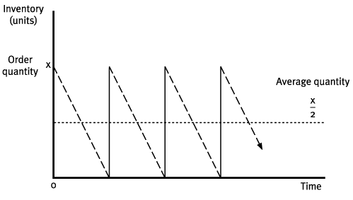
If x is the quantity ordered, the annual holding cost would be calculated as:

Holding cost per unit × Average inventory:

We therefore see an upward sloping, linear relationship between the re-order quantity and total annual holding costs.

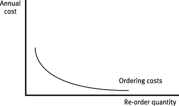
Ordering costs

The model assumes that a fixed cost is incurred every time an order is placed (referred to as C_Oin the formula). Therefore, as the order quantity increases, there is afall in the number of orders required, which reduces the total orderingcost.

If D is the annual expected sales demand, the annual order cost is calculated as:

Order cost per order × no. of orders per annum.

However, the fixed nature of the cost results in a downward sloping, curved relationship.

Because you are trying to balance these two costs (one whichincreases as re-order quantity increases and one which falls), totalcosts will always be minimised at the point where the total holdingcosts equals the total ordering costs. This point will be the economicorder quantity.

When the re-order quantity chosen minimises the total cost of holding and ordering, it is known as the EOQ.

Assumptions

The following assumptions are made:

• demand and lead time are constant and known
• purchase price is constant
• no buffer inventory held (not needed).

These assumptions are critical and should be discussed when consideringthe validity of the model and its conclusions, e.g. in practice, demandand/or lead time may vary.

The calculation

The EOQ can be more quickly found using a formula (given in the examination):

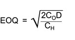
where:

C_O = cost per order

D = annual demand

C_H = cost of holding one unit for one year.

Test your understanding 1 – EOQ I

A company requires 1,000 units of material X per month. The costper order is $30 regardless of the size of the order. The holding costsare $2.88 per unit pa.

Required:

Investigate the total cost of buying the material in quantities of400, 500, or 600 units at one time. What is the cheapest option?

Use the EOQ formula to prove your answer is correct.

Test your understanding 2 – EOQ II

Monthly demand for a product is 10,000 units. The purchase price is$10/unit and the company's cost of finance is 15% pa. Warehouse storagecosts per unit pa are $2/unit. The supplier charges $200 per order fordelivery.

Calculate the EOQ.

Dealing with quantity discounts

Discounts may be offered for ordering in large quantities. If theEOQ is smaller than the order size needed for a discount, should theorder size be increased above the EOQ?

To work out the answer you should carry out the following steps:

Step 1: Calculate EOQ, ignoring discounts.

Step 2: If the EOQ is below the quantity qualifying for adiscount, calculate the total annual inventory cost arising from usingthe EOQ.

Step 3: Recalculate total annual inventory costs using the order size required to just obtain each discount.

Step 4: Compare the cost of Steps 2 and 3 with the saving from the discount, and select the minimum cost alternative.

Step 5: Repeat for all discount levels.

Test your understanding 3 – EOQ with discounts I

W Co is a retailer of barrels. The company has an annual demand of30,000 barrels. The barrels cost $2 each. Fresh supplies can be obtainedimmediately, with ordering and transport costs amounting to $200 perorder. The annual cost of holding one barrel in stock is estimated to be$1.20.

A 2% discount is available on orders of at least 5,000 barrels and a2.5% discount is available if the order quantity is 7,500 barrels orabove.

Required:

Calculate the EOQ ignoring the discount and determine if it would change once the discount is taken into account.

Test your understanding 4 – EOQ with discounts II

D Co uses component V22 in its construction process. The companyhas a demand of 45,000 components pa. They cost $4.50 each. There is nolead time between order and delivery, and ordering costs amount to $100per order. The annual cost of holding one component in inventory isestimated to be $0.65.

A 0.5% discount is available on orders of at least 3,000 componentsand a 0.75% discount is available if the order quantity is 6,000components or above.

Calculate the optimal order quantity.

3 Calculating the re-order level (ROL)

Known demand and lead time

Having decided how much inventory to re-order, the next problem iswhen to re-order. The firm needs to identify a level of inventory whichcan be reached before an order needs to be placed.

The ROL is the quantity of inventory on hand when an order is placed.

When demand and lead time are known with certainty the ROL may be calculated exactly, i.e. ROL = demand in the lead time.

Test your understanding 5 – Calculating the re-order level I

Using the data for W Co, assume that the company adopts the EOQ asits order quantity and that it now takes two weeks for an order to bedelivered.

How frequently will the company place an order? How much inventory will it have on hand when the order is placed?

Test your understanding 6 – Calculating the re-orderlevel II

Using the data relating to D Co, and ignoring discounts, assumethat the company adopts the EOQ as its order quantity and that it nowtakes three weeks for an order to be delivered.

(a)How frequently will the company place an order?

(b)How much inventory will it have on hand when the order is placed?

ROL with variable demand or variable lead time

When lead time and demand are known with certainty, ROL = demandduring lead time. Where there is uncertainty, an optimum level of bufferinventory must be found. This depends on:

• variability of demand
• cost of holding inventory
• cost of stockouts.

You will not be required to perform this calculation in the examination.

Re-order levels

If there were certainty, then the last unit of inventory would besold as the next delivery is made. In the real world, this ideal cannotbe achieved. Demand will vary from period to period, and ROL must allowsome buffer (or safety) inventory, the size of which is a function ofmaintaining the buffer (which increases as the levels increase), runningout of inventory (which decreases as the buffer increases) and theprobability of the varying demand levels.

4 Inventory management systems

A number of systems have been developed to simplify the inventory management process:

• bin systems
• periodic review
• JIT.

Bin systems

A simple visual reminder system for re-ordering is to use a bin system.

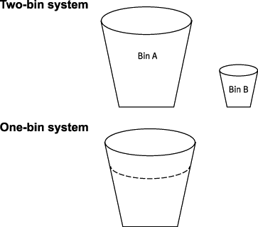
Two-bin system

This system utilises two bins, e.g. A and B. Inventory is takenfrom A until A is empty. An order for a fixed quantity is placed and, inthe meantime, inventory is used from B. The standard inventory for B isthe expected demand in the lead time (the time between the order beingplaced and the inventory arriving), plus some 'buffer' inventory.

When the new order arrives, B is filled up to its standard leveland the rest is placed in A. Inventory is then drawn as required from A,and the process is repeated.

One-bin system

The same sort of approach is adopted by some firms for a single bin with a red line within the bin indicating the ROL.

These methods rely on accurate estimates of:

• lead time
• demand in lead time.

Action must therefore be taken if inventory levels:

• fall below a preset minimum
• exceed a preset maximum.

Control levels

Minimum inventory level usually corresponds with buffer inventory.If inventory falls below that level, emergency action to replenish maybe required.

Maximum inventory level would represent the normal peak holding,i.e. buffer inventory plus the re-order quantity. If the maximum isexceeded, a review of estimated demand in the lead time is needed.

The levels would also be modified according to the relative importance/cost of a particular inventory item.

Periodic review system (constant order cycle system)

Inventory levels are reviewed at fixed intervals, e.g. every fourweeks. The inventory in hand is then made up to a predetermined level,which takes account of:

• likely demand before the next review
• likely demand during the lead time.

Thus a four-weekly review in a system where the lead time was twoweeks would demand that inventory be made up to the likely maximumdemand for the next six weeks.

Additional question - Periodic review systems

A company has estimated that for the coming season weekly demandfor components will be 80 units. Suppliers take three weeks on averageto deliver goods once they have been ordered and a buffer inventory of35 units is held.

If the inventory levels are reviewed every six weeks, how manyunits will be ordered at a review where the count shows 250 units ininventory?

The answer to this question can be found after the chapter summary diagram at the end of this chapter.

Bin systems versus periodic review

Slow moving inventory

Certain items may have a high individual value, but be subject to infrequent demand.

In most organisations, about 20% of items held make up 80% of total usage (the 80/20 rule).

Slow-moving inventory

Management need to review inventory usage to identify slow-movinginventory. An aged inventory analysis should be produced and reviewedregularly so that action can be taken. Actions could include:

• elimination of obsolete items
• slow-moving inventory items only ordered when actually needed (unless a minimum order quantity is imposed by the supplier)
• review of demand level estimates on which re-order decisions are based.

A regular report of slow-moving items is useful in that managementis made aware of changes in demand and of possible obsolescence.Arrangements may then be made to reduce or eliminate inventory levelsor, on confirmation of obsolescence, for disposal.

Just in Time (JIT) systems

JIT is a series of manufacturing and supply chain techniques that aimto minimise inventory levels and improve customer service bymanufacturing not only at the exact time customers require, but also inthe exact quantities they need and at competitive prices.

In JIT systems the balancing act is dispensed with. Inventory is reduced to an absolute minimum or eliminated altogether.

Aims of JIT are:

• a smooth flow of work through the manufacturing plant
• a flexible production process which is responsive to the customer's requirements
• reduction in capital tied up in inventory.

This involves the elimination of all activities performed that do not add value = waste.

Just in time systems

JIT extends much further than a concentration on inventory levels.It centres around the elimination of waste. Waste is defined as anyactivity performed within a manufacturing company which does not addvalue to the product. Examples of waste are:

• raw material inventory
• WIP inventory
• finished goods inventory
• materials handling
• quality problems (rejects and reworks, etc.)
• queues and delays on the shop floor
• long raw material lead times
• long customer lead times
• unnecessary clerical and accounting procedures.

JIT attempts to eliminate waste at every stage of the manufacturing process, notably by the elimination of:

• WIP, by reducing batch sizes (often to one)
• raw materials inventory, by the suppliers delivering direct to the shop floor JIT for use
• scrap and rework, by an emphasis on total quality control of the design, of the process, and of the materials
• finished goods inventory, by reducing lead times so that all products are made to order
• material handling costs, by re-design of the shop floor so that goods move directly between adjacent work centres.

The combination of these concepts in JIT results in:

• a smooth flow of work through the manufacturing plant
• a flexible production process which is responsive to the customer's requirements
• reduction in capital tied up in inventory.

A JIT manufacturer looks for a single supplier who can provide high quality, frequent and reliable deliveries, rather than the lowest price. In return, the supplier can expect more business under long-term purchase orders, thus providing greater certainty in forecasting activity levels. Very often the suppliers will be located close to the company.

Long-term contracts and single sourcing strengthen buyer-supplierrelationships and tend to result in a higher quality product. Inventoryproblems are shifted back onto suppliers, with deliveries being made asrequired.

The spread of JIT in the production process inevitably affectsthose in delivery and transportation. Smaller, more frequent loads arerequired at shorter notice. The haulier is regarded as almost a partnerto the manufacturer, but tighter schedules are required of hauliers,with penalties for non-delivery.

Reduction in inventory levels reduces the time taken to countinventory and the clerical cost. However with JIT, although inventoryholding costs are close to zero, inventory ordering costs are high.

You need to be able to outline the key features of each stock controlsystem and the impact they may have on ordering and holding costs and/ororder dates and quantities. Ensure you can discuss the implications ofJIT for production processes and supplier relationships as well asinventory levels.

Chapter summary

Answer to additional question - Periodic review systems

Demand per week is 80 units. The next review will be in six weeks by which time 80 × 6 = 480 units will have been used.

An order would then be placed and during the lead time – three weeks – another 80 × 3 = 240 units will be used.

The business therefore needs to have 480 + 240 = 720 units ininventory to ensure a stockout is avoided. Since buffer inventory of 35units is required, the total number needed is 755 units.

Since the current inventory level is 250 units, an order must be placed for 755 – 250 = 505 units.

Test your understanding answers

Test your understanding 1 – EOQ I

Solution:

Therefore the best option is to order 500 units each time.

Note: that this is the point at which total cost is minimised and the holding costs and order costs are equal.

Solution using the formula:

C_O = 30

D = 1,000 × 12 = 12,000

C_H = 2.88

Test your understanding 2 – EOQ II

C_O = $200

D = 10,000 units × 12 = 120,000 units per annum

C_H = (10 × 0.15) + 2 = $3.5 per unit per annum

Test your understanding 3 – EOQ with discounts I

Solution

Step 1 Calculate EOQ, ignoring discounts.

C_O = $200

D = 30,000 barrels per annum

C_H = $1.20 per barrel per annum

Step 2 As this is below the level for discounts, calculate total annual inventory costs.

Total annual costs for the company will comprise holding costs plus re-ordering costs.

Step 3 Recalculate total annual inventory costs using the order size required to just obtain the discount.

At order quantity 5,000, total costs are as follows.

Hence batches of 5,000 are worthwhile.

Step 3 (again)

At order quantity 7,500, total costs are as follows:

So a further cost saving cannot be made on orders of 7,500 units.The company should therefore opt for buying 5,000 units in order tomaximise the benefit.

Note: If Step 1 produces an EOQ at which a discount would havebeen available, and the holding cost would be reduced by taking thediscount, i.e. where C_H is based on the purchase price × the cost of finance, the EOQ must be recalculated using the new C_H before the above steps are followed.

Test your understanding 4 – EOQ with discounts II

Step 1

C_O = $100 per order

D = 45,000 components per annum

C_H = $0.65 per component per annum

Step 2

Total annual costs for the company will comprise holding costs plus re-ordering costs.

= (Average inventory × C_H) + (Number of re-orders pa × C_O)

= $2,419 per annum

Step 3

At an order quantity of 6,000 components, total costs are as follows.

(6,000 × $0.65/2) + (45,000 × $100 ÷ 6,000) = $2,700

So a saving can be made on orders of 6,000 components.

Test your understanding 5 – Calculating the re-orderlevel I

• Annual demand is 30,000. The original EOQ is 3,162 barrels per order. The company will therefore place an order once every

• The company must be sure that there is sufficient inventory on hand when it places an order to last the two weeks' lead time. It must therefore place an order when there is two weeks' worth of demand in inventory:

Test your understanding 6 – Calculating the re-orderlevel II

(a)Annual demand is 45,000 components. The original EOQ is 3,721 components per order.

The company will therefore place an order once every
3,721 ÷ 45,000 × 365 days = 30 days

(b)The company must be sure thatthere is sufficient inventory on hand when it places an order to lastthe three weeks’ lead time. It must therefore place an order when thereis three weeks’ worth of demand in inventory:

3/52 × 45,000 = 2,596 components in inventory.

Rating :	Ratings & Comments  (Click the stars to rate the page)

Tags: